Introduction

The bias-variance tradeoff is a fundamental property of machine learning models, and is critical for performance evaluation and model selection. It relates statistical quantities of bias and variance to two central modeling deficiencies: underfitting and overfitting.

We will first prove that the expected mean squared error (MSE) of a regression problem can be refactored into a more familiar and interpretable form with the bias-variance decomposition. Then, we will introduce a classic framework in which we can better understand the bias-variance tradeoff, and learn about how it relates to underfitting and overfitting. We will end with discussions of regularization and how deep learning fits into the picture.

Formulation

Let $y(x) = f(x) + \epsilon$ be the observed relationship where $f$ is the true (unknown) population relationship, and let $\hat{y} = g(x)$ be the model predicted value for input $x$ whose ground truth label is $y$. Let $g$ be a model trained on a given training set $S \sim D$ where $D$ is the base distribution from which data is generated. The mean squared error (MSE) of the regression model over a given test set with i.i.d. samples $\tilde{S} = \{x_i | i = 1, \dots, t\} \sim D$ is given by $ \DeclareMathOperator{\EX}{\mathbf{E}} % expected value $ $\newcommand{\indep}{\perp \!\!\! \perp} % independence $

\[\text{MSE}_{\tilde{S}} = \frac{1}{t} \sum_{i=1}^{t} \big(f(x_i) + \epsilon_i - g(x_i)\big)^2\]

where $\epsilon_i$ is the intrinsic noise (a.k.a. irreducible error or Bayes error) associated with the test observation $x_i$ and we can assume:

$(1)$ $\epsilon_i$ is independent of the training ($S$) and test ($\tilde{S}$) sets, therefore it is independent of the trained model $g$ and the test observation $x_i$.

$(2)$ $\epsilon_i$ is sampled from a $0$-mean distribution $\mathscr{E}$: $\EX_{\epsilon \sim \mathscr{E}}{[\epsilon_i]} = 0 $.

$(3)$ $f$ is a deterministic (i.e. not a random variable) function and can be treated as a constant; it does not change with the randomness in the sampling of the training set.

Using the given problem definition and facts, we would like to prove the following statement:

\[\EX{[\text{MSE}]} = \text{Bias}^2 + \text{Variance} + \text{Noise}\]

Proof

The expected value (over the randomness in the choice of different training sets and different $\epsilon$) of the mean squared error (on the same test set $\tilde{S}$), is given by:

\[\begin{align*} \EX{\left[\text{MSE}_{\tilde{S}}\right]} &= \EX_{S \sim D, \epsilon \sim \mathscr{E}}{\left[\text{MSE}_{\tilde{S}}\right]}\\ &= \EX{\left[\frac{1}{t} \sum_{i=1}^{t} \big(f(x_i) + \epsilon_i - g(x_i)\big)^2\right]} \\ &= \frac{1}{t} \sum_{i=1}^{t} \EX{\left[\big(f(x_i) + \epsilon_i - g(x_i)\big)^2 \right]} \quad \text{by linearity of expectation} \\ &= \frac{1}{t} \sum_{i=1}^{t} \big(\EX{\big[f^{2}(x_i)\big]} + \EX{\big[2 \epsilon_i f(x_i) \big]} + \EX{\big[\epsilon_{i}^{2} \big]} - \EX{\big[2 f (x_i) g(x_i)\big]} - \EX{\big[2 \epsilon_i g(x_i) \big]} + \EX{\big[g^2(x_i) \big]} \big) \\ &\quad \: \text{by linearity of expectation} \\ &= \frac{1}{t} \sum_{i=1}^{t} \big(\EX{\big[f^{2}(x_i)\big]} + 2\EX{[\epsilon_i]}\EX{[f(x_i)]} + \EX{\big[\epsilon_{i}^{2} \big]} - \EX{\big[2 f (x_i) g(x_i)\big]} - 2\EX{[\epsilon_i]}\EX{[g(x_i)]} + \EX{\big[g^2(x_i) \big]} \big)\\ & \quad \: \text{by } (1) \text{ and } X \indep Y \iff \EX{[XY]} = \EX{[X]} \EX{[Y]} \\ &= \frac{1}{t} \sum_{i=1}^{t} \left(\EX{\big[f^{2}(x_i)\big]} + \EX{\big[\epsilon_{i}^{2} \big]} - \EX{\big[2 f (x_i) g(x_i)\big]} + \EX{\big[g^2(x_i) \big]} \right) \quad \text{by } (2)\\ &= \frac{1}{t} \sum_{i=1}^{t} \EX{\big[\big(f(x_i) - g(x_i)\big)^2 \big]} + \frac{1}{t} \sum_{i=1}^{t} \EX{\big[\epsilon_{i}^{2} \big]} \\ & \quad \: \text{by square collapse and linearity of expectation} \\ &= \frac{1}{t} \sum_{i=1}^{t} \EX{\bigg[\bigg(\big(f(x_i) - \EX{[g(x_i)]}\big) + \big(\EX{[g(x_i)]} - g(x_i)\big)\bigg)^2 \bigg]} + \frac{1}{t} \sum_{i=1}^{t} \EX{\big[\epsilon_{i}^{2} \big]} \\ & \quad \: \text{by } (a-b)^2 = \big((a-c) + (c-b)\big)^2 \\ &= \frac{1}{t} \sum_{i=1}^{t} \EX{\big[\big(f(x_i) - \EX{[g(x_i)]}\big)^2\big]} \\ &\quad + \frac{2}{t} \sum_{i=1}^{t} \EX{\big[\big(f(x_i) - \EX{[g(x_i)]}\big)\big(\EX{[g(x_i)]} - g(x_i)\big)\big]} \\ & \quad + \frac{1}{t} \sum_{i=1}^{t} \EX{\big[\big(\EX{[g(x_i)]} - g(x_i)\big)^2\big]} \\ & \quad + \frac{1}{t} \sum_{i=1}^{t} \EX{\big[\epsilon_{i}^{2} \big]} \quad \text{by square expansion} \end{align*}\]

We can rewrite the second term as

\[\frac{2}{t} \sum_{i=1}^{t} \EX{\big[\big(f(x_i) - \EX{[g(x_i)]}\big)\big(\EX{[g(x_i)]} - g(x_i)\big)\big]} = \frac{2}{t} \sum_{i=1}^{t} \bigg(\big(f(x_i) - \EX{[g(x_i)]}\big) \EX{\big[\EX{[g(x_i)]} - g(x_i)\big]}\bigg)\]

by distributing the expectation inside because

$(4)$ $\big(f(x_i) - \EX{[g(x_i)]}\big)$ is deterministic (i.e. not a random variable) and can be treated as a constant. This is by $(3)$ and because $\EX{[\cdot]}$ returns a constant.

Moreover, notice that

\[\EX{\big[\EX{[g(x_i)]} - g(x_i)\big]} = \EX{\big[\EX{[g(x_i)]}\big]} - \EX{[g(x_i)]} = \EX{[g(x_i)]} - \EX{[g(x_i)]} = 0\]

first by linearity of expectation and then by both terms being constant.

Therefore, the second term evaluates to $0$ and we can simplify the objective expectation to

\[\begin{align*} \EX{\left[\text{MSE}_{\tilde{S}}\right]} & = \frac{1}{t} \sum_{i=1}^{t} \EX{\big[\big(f(x_i) - \EX{[g(x_i)]}\big)^2\big]} + \frac{1}{t} \sum_{i=1}^{t} \EX{\big[\big(\EX{[g(x_i)]} - g(x_i)\big)^2\big]} + \frac{1}{t} \sum_{i=1}^{t} \EX{\big[\epsilon_{i}^{2} \big]} \\ &= \underbrace{\frac{1}{t} \sum_{i=1}^{t} \big(\EX{[g(x_i)]} - f(x_i)\big)^2}_{\text{Bias}^2} + \underbrace{\frac{1}{t} \sum_{i=1}^{t} \EX{\big[\big(g(x_i) - \EX{[g(x_i)]}\big)^2\big]}}_{\text{Variance}} + \underbrace{\frac{1}{t} \sum_{i=1}^{t} \EX{\big[\epsilon_{i}^{2} \big]}}_{\text{Noise}} \\ & \quad \: \text{by } (a-b)^2 = (b-a)^2 \text{ and (4)} \\ \end{align*}\]

This assignments above are by definition. The bias and the variance of an estimate $\skew{1}\hat{\theta}$ of an statistical parameter whose true population value is $\theta$, or respectively $\hat{y}$ and $y$ in our case, are given by: $ \DeclareMathOperator{\Var}{\mathrm{Var}} % variance $ $ \DeclareMathOperator{\Bias}{\mathrm{Bias}} % bias $

\[\begin{align*} \Bias_{\theta}(\skew{1}\hat{\theta}) &= \EX{[\skew{1}\hat{\theta} - \theta]} = \EX{[\skew{1}\hat{\theta}]} - \theta \\ \Var(\skew{1}\hat{\theta}) &= \EX{\big[\big(\skew{1}\hat{\theta} - \EX{[\skew{1}\hat{\theta}]}\big)^2\big]} \\ \end{align*}\]

Notice that the $\text{Noise}$ above is not the same as the intrinsic noise we started with in $y(x)$, which was $\epsilon$. Whereas $\epsilon$ is often a random variable defined over a distribution (e.g. $\mathscr{N}(0, 0.3)$), the $\text{Noise}$ we end up with is a constant. More specifically:

\[\text{Noise} = \frac{1}{t} \sum_{i=1}^{t} \EX{\big[\epsilon_{i}^{2} \big]} = \frac{t \EX{\big[\epsilon_{i}^{2} \big]}}{t} = \EX{\big[\epsilon_{i}^{2} \big]} = \EX{\big[(\epsilon_i - \mu_{\epsilon_i})^2\big]} = \Var{[\epsilon_i]} = \sigma_{\epsilon}^2\]

where $\mu_{\epsilon_i} = \EX{[\epsilon_i]} = 0$ from $(2)$. Therefore, $\text{Noise}$ is the variance of the intrinsic noise under the assumption of $(2)$.

Finally, we should note that we have worked on the conditional expectation of the mean-squared error, i.e. computing it on a specific test set $\tilde{S}$, up until now. Unconditionally, i.e. taking the expectation over all possible test sets, the bias-variance decomposition yields: $ \DeclareMathOperator{\d}{\mathrm{d} \!} % a small nudge, differential operator $

\[\EX{\left[\text{MSE}\right]} = \int{\text{Bias}^2\big(g(x)\big) D(\d x)} + \int{\text{Var}\big(g(x)\big) D(\d x)} + \sigma_{\epsilon}^2\]

where $D$ is the base distribution from which data is generated as previously defined.

\[\tag*{Q.E.D.}\]

Discussion

Estimation Bias and Estimation Variance

The bias and the variance are two sources of estimation error for any fitted model $g$ (or sometimes shown as $\hat{f}$) as shown in the proof.

If the fitted model belongs to a model class that is far from the true relationship $f$ (e.g. we fit a linear model whereas the true relationship is exponential), we incur estimation bias.

If the fitted model is highly variable, we end up with substantially different models over different training instances (e.g. different subsets of data, shuffling data with different random seeds, etc.), and incur estimation variance. For instance, this might happen if a model fits to the noise in the data.

Classical U-shaped Curve in Bias-Variance Tradeoff

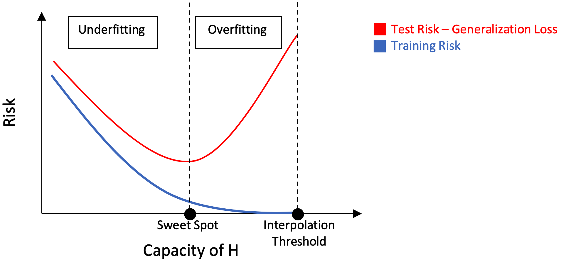
The classical U-shaped curve has been a textbook mental model to guide model selection in the machine learning literature. The classical thinking is concerned with finding the sweet spot between underfitting and overfitting as shown in the figure above, where the x-axis is the empirical risk or loss and y-axis is the capacity of a model class $H$. The capacity here can be thought of as the complexity of the model (e.g. number of model parameters).

Whereas underfitting region has high bias but low variance, overfitting region has high variance but low bias. This poses the bias-variance tradeoff. Check [1] to see this tradeoff at play.

When the class capacity is increased sufficiently, the model perfectly fits to the training data (i.e. interpolation). The capacity at which interpolation is achieved is known as the interpolation threshold, and is characterized by an optimal or near-optimal training risk. For capacities smaller than this threshold, the learned predictors exhibit the shown classical U-shaped curve.

(Optional) Regularization

The goal of regularization is to improve the generalization of a model by reducing its complexity. The $\ell_p$-norm regularization technique is one such method. Regularization makes a model perform well on test data often at the expense of its performance on training data. Therefore, it avoids overfitting by increasing bias and reducing variance. Often times, for regularization to work as desired, we need to tune a regularization strength parameter.

(Optional) Double Descent Curve

Modern machine learning methods (e.g. deep neural networks) have high capacity ($ H \to \infty$), and are fit perfectly (i.e. interpolation) to the training data. However, they achieve significantly lower errors on test data. Motivated by how this is in contrast with the classical thinking, which would classify these models as overfitting instead, [4] proposes the double descent risk curve as shown in the figure above.

It is an extension to the classical U-shaped curve, and it adds to the story significantly: although we observe an increasing and diverging risk at the interpolation threshold, increasing capacity beyond this point yields decreasing risk, and therefore complex models (which usually have number of features $d$ $\geq$ number of data points $n$) end up achieving better generalization compared to simpler models stopped at the sweet spot of the Classical Regime. This is shown by the second descent in the graph.

References

[1] Dustin Stanbury’s Blog

[2] Columbia University, COMS 6998: Practical Deep Learning Systems Performance, Prof. Parijat Dube

[3] Chapter 4 of Neural Networks and Deep Learning by Charu C. Aggarwal

[4] Mikhail Belkin, Daniel Hsu, Siyuan Ma, & Soumik Mandal. (2019). Reconciling modern machine learning practice and the bias-variance trade-off.