
Basics of Unconstrained Optimization
Tags: optimization numerical-methods
Introduction
Optimization is an essential tool in decision science, and it is widely applicable to many fields thanks to its application-agnostic definition. Optimization is integral to humans and their understanding of the world in many ways. For example, investors seek to create portfolios that achieve high rates of return, manufacturers and civil engineers aim for maximum efficiency in their design, and engineers adjust parameters to optimize the performance of their algorithms.
In this post, we will (i) cover the fundamentals of unconstrained optimization of smooth functions, (ii) formulate and implement a few popular optimization algorithms in Python, (iii) and end with a comparative analysis and discussion. The ideas and algorithms described in this post are highly relevant to the bigger world of numerical methods.
Imports
%matplotlib inline
%precision 16

import numpy as np
import pandas as pd
from scipy.optimize import rosen, rosen_der, rosen_hess

import matplotlib
from matplotlib import cm
from matplotlib.patches import Circle
import matplotlib.pyplot as plt
plt.rcParams["font.size"] = 12
Formulation
Optimization is the maximization or minimization of an objective function $f$, potentially subject to constraints $c$ on some variables $x$. A mathematical convenience that arises is that to maximize $f$ is to minimize $-f$ and vice versa. Throughout this post, we will focus on multivariate minimization.
Unconstrained optimization algorithms either require the user to specify the starting point $x_0$ based on some prior knowledge, or choose $x_0$ by a systematic approach. These algorithms follow the general pseudocode given below:
- Begin at $x_0$
- Generate a sequence of iterates $\{x_k\}_{k=0}^\infty$
- Use information about $f$ at $x_k$ and possibly at earlier iterates $x_0, \ldots, x_{k-1}$ to decide on $x_{k+1}$
- Find a $x_{k+1}$ such that $f(x_{k+1}) < f(x_k)$
- Repeat
- Terminate when no more progress can be made or a solution point has been approximated with sufficient accuracy
There are two main strategies for moving from the current point $x_k$ to a new iterate $x_{k+1}$ in an optimization algorithm: line search and trust region. They differ in the order in which they choose the direction and distance of the move to the next iterate.
Line Search
The algorithm chooses a direction $p_k$ and searches along it for a new iterate with a lower function value. The distance to move along $p_k$ is found by solving for the step length $\alpha$ in the following minimization subproblem:
\[\underset{\alpha > 0}{\min} f(x_k + \alpha p_k)\]Solving this exactly would derive the maximum benefit from the direction $p_k$, but an exact minimization is expensive and usually unnecessary. Instead, the algorithm can generate a limited number of trial step lengths until it finds one that loosely approximates the minimum in each step.
Trust Region
The algorithm uses information gathered about $f$ to construct a model function $m_k$ which behaves similar to $f$ near the current point $x_k$. However, by definition, $m_k$ might not approximate $f$ well when $x$ is far from $x_k$. Therefore, we can restrict the search to some region around $x_k$. The candidate step $p$ can then be found by solving the following minimization subproblem:
\[\underset{p}{\min} m_k(x_k + p) \quad \text{where } x_k + p \text{ lies inside the trust region}\]The algorithms we will cover here will employ the line search strategy. Before introducing and implementing these algorithms, let’s first take a look at line search conditions and a related routine for picking a reasonable step length $\alpha$ at each time step. We will use this same routine for each line search algorithm introduced later.
Step Length
There is a fundamental tradeoff when choosing the step length $a_k$. We want a substantial reduction of $f$, yet we cannot afford to spend too much time making a choice. In general, it is very expensive to identify the $\alpha$ that would yield a global or even local minimizer. The computational complexity arises from the increasing number of function evaluations. Then, instead of an exact line search, most methods use a bracketing phase to find a reasonable interval and an interpolation phase to compute a good step length within this interval. Due to this inexact nature, line search algorithms have various termination conditions as discussed next.
Wolfe Conditions
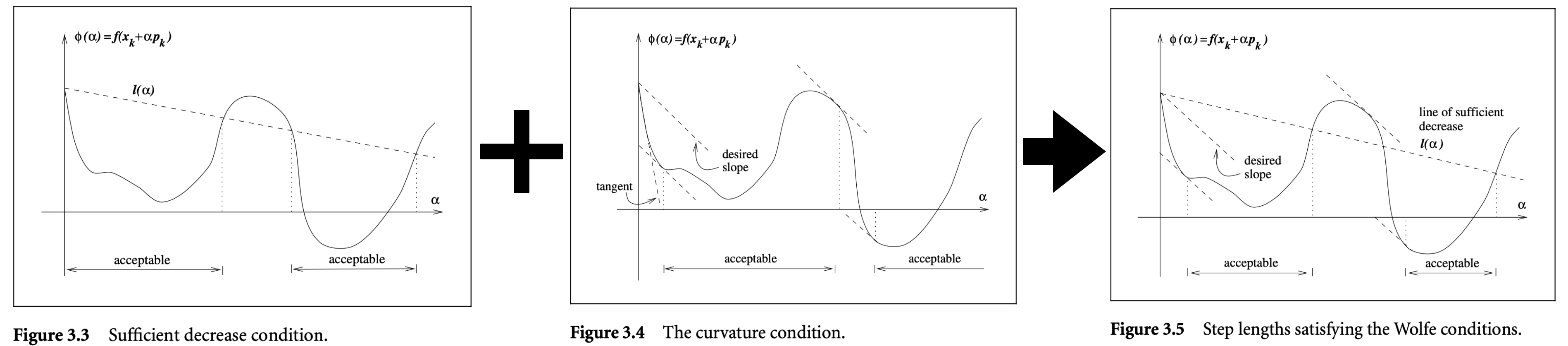
Sufficient Decrease Condition
The sufficient decrease condition states that a reasonable step length $\alpha_k$ should yield a sufficient decrease in $f$, denoted by:
\[f(x_k + \alpha p_k) \leq f(x_k) + c_1 \alpha \nabla f_k^T p_k \quad \text{for some constant } c_1 \in (0, 1)\]where $c_1$ is chosen to be quite small, say $c_1 = 10^{-4}$, in practice.
Curvature Condition
The sufficient decrease condition is not enough by itself to ensure that the algorithm makes reasonable progress as it is satisfied for all sufficiently small values of $\alpha$ (see figure below). Therefore, the curvature condition rules out short step lengths by stating:
\[|\nabla f(x_k + \alpha_k p_k)^T p_k| \geq c_2 |\nabla f_k^T p_k| \quad \text{for some constant } c_2 \in (c_1, 1)\]where typical values of $c_2$ are $c_2 = 0.9$ when the search direction $p_k$ is chosen by a Newton or quasi-Newton method, and $c_2 = 0.1$ when $p_k$ is obtained from a nonlinear conjugate gradient method.
When both the sufficient decrease and curvature conditions are satisfied, it is said that the strong Wolfe conditions are satisfied. Below figure taken from [1] shows this.
There is a one-dimensional search procedure that is guaranteed to find a step length satisfying the strong Wolfe conditions for any parameters $c_1$ and $c_2$ such that $0 < c_1 < c_2 < 1$. The procedure has two stages:
- The first stage begins with a trial estimate $\alpha_1$ and keeps increasing until an acceptable step length or interval for bracketing is found.
- The second stage employs interpolation and successively decreases the size of the interval until an acceptable step length is identified.
Let’s now implement this procedure alongside its prerequisites (e.g. line search conditions) ahead of time as it will come in handy later.
def satisfies_sufficient_decrease(f, gradient, xk, alpha, pk, c1=1e-4):
    """Implements the sufficient decrease condition as described above."""
    assert 0.0 < c1 < 1.0
    return f(xk + alpha * pk) <= f(xk) + c1 * alpha * gradient(xk).dot(pk)


def satisfies_curvature(f, gradient, xk, alpha, pk, c2=0.9):
    """Implements the curvature condition as described above."""
    assert 0.0 < c2 < 1.0
    return abs(gradient(xk + alpha * pk).dot(pk)) <= c2 * abs(gradient(xk).dot(pk))


def satisfies_strong_wolfe(f, gradient, xk, alpha, pk, c1=1e-4, c2=0.9):
    """Implements the strong Wolfe conditions as described above."""
    assert 0.0 < c1 < c2 < 1.0
    return satisfies_sufficient_decrease(f, gradient, xk, alpha, pk, c1) and \
           satisfies_curvature(f, gradient, xk, alpha, pk, c2)


def interpolation(f, gradient, f_alpha, gradient_alpha, alpha,
                  c1, c2, satisfies_strong_wolfe_alpha, iters=20):
    """
    Implements the second stage: interpolation of the line search step length
    finding routine. This routine is modified from a class example [6].
    """
    low, high = 0.0, 1.0

    for i in range(iters):
        if satisfies_strong_wolfe_alpha(f, gradient, alpha, c1, c2):
            return alpha

        middle = (low + high) / 2

        numerator = -gradient_alpha(low) * (high ** 2)
        denominator = 2 * (f_alpha(high) - f_alpha(low) - gradient_alpha(low) * high)
        alpha = numerator / denominator

        if alpha < low or alpha > high:
            alpha = middle

        if gradient_alpha(alpha) > 0:
            high = alpha
        elif gradient_alpha(alpha) <= 0:
            low = alpha

    return alpha

def find_step_length(f, gradient, xk, alpha, pk, c1=1e-4, c2=0.9, iters=20):
    """
    Implements the line search step length finding algorithm for satisfying
    strong Wolfe conditions as discussed above.
    """
    satisfy = lambda f, gradient, alpha, c1, c2: satisfies_strong_wolfe(f,
                                                                        gradient,
                                                                        xk,
                                                                        alpha,
                                                                        pk,
                                                                        c1,
                                                                        c2)
    return interpolation(f,
                         gradient,
                         lambda alpha: f(xk + alpha * pk),
                         lambda alpha: gradient(xk + alpha * pk).dot(pk),
                         alpha,
                         c1,
                         c2,
                         satisfy,
                         iters)
The following error calculation code will also come in handy while measuring the performance of optimization algorithms.
def errors(f, F, reduction='mean', eps=np.finfo(float).eps):
    """
    Calculates various measures of error of an object f and its approximation F

    :param (np.ndarray) f: float array of true values
    :param (np.ndarray) F: float array of approximate values
    :param (str or None) reduction: reduction technique (i.e. to scalar) on error arrays
    :param (float) eps: epsilon value to prevent divison by 0 errors
    :returns:
        e: array of absolute errors
        r: array of relative errors
        p: integer array of precisions
    """
    # Convert the inputs to NumPy array (only effective when the input type is float)
    f, F = np.array(f) + eps, np.array(F)

    e = np.abs(f - F)
    r = e / np.abs(f)
    p = np.log10(5/r).astype(int)

    if reduction == 'mean':
        return np.mean(e), np.mean(r), np.mean(p)
    elif reduction == 'sum':
        return np.sum(e), np.sum(r), np.sum(p)
    elif reduction is None:
        return e, r, p
    else:
        raise ValueError('reduction=%s is not recognized!' % reduction)
Algorithms
Steepest Descent Method
The steepest descent direction, $-\nabla f_k$ is the direction along which $f$ decreases most rapidly and is consequently the most obvious choice for the search direction of a line search strategy. To prove this, let’s introduce Taylor’s Theorem.
Taylor Series and subsequently Taylor’s Theorem is one of the most powerful tools mathematics has to offer for approximating a function. For a vector-valued function, we can state it as follows: $ \DeclareMathOperator{\D}{\mathop{\: \mathrm{d}}} % differential $
\[\begin{align*} &\text{If } f: \mathbb{R}^n \to \mathbb{R} \text{ is continuously differentiable and } p \in \mathbb{R}^n \text{:} \\ &f(x + p) = f(x) + \nabla f (x + tp)^T p \quad \text{for some } t \in (0, 1) \\ &\text{If } f \text{ is twice continously differentiable:} \\ &\nabla f(x + p) = \nabla f(x) + \int_{0}^{1} \nabla^2 f(x + tp)p \D{t} \quad \text{and} \\ &f(x + p) = f(x) + \nabla f(x)^T p + \frac{1}{2} p^T \nabla^2 f(x + tp)p \quad \text{for some } t \in (0, 1) \\ \end{align*}\]Taylor’s Theorem tells us that for any search direction $p$ and step length $\alpha$, we have:
\[f(x_k + \alpha p) = f(x_k) + \alpha p^T \nabla f_k + \frac{1}{2} \alpha^2 p^T \nabla^2 f(x_k + tp)p \quad \text{for some } t \in (0, 1)\]The rate of change in $f$ along direction $p$ at $x_k$ then becomes the coefficient of $\alpha$, namely $p^T \nabla f_k$. The unit direction $p$ of the most rapid decrease can be found by solving the following minimization subproblem:
\[\begin{align*} &\underset{p}{\min} p^T \nabla f_k \quad \text{ subject to} ||p|| = 1 \\ & = \underset{p}{\min} ||p|| ||\nabla f_k|| \cos \theta \quad \text{by } a \cdot b = ||a|| ||b|| \cos \theta \\ & = \underset{p}{\min} ||\nabla f_k || \cos \theta \quad \text{by } ||p|| = 1 \\ \end{align*}\]The minimizer is attained when $\cos \theta = -1$, and $\theta$ here denotes the angle between $p$ and $\nabla f_k$. This yields:
\[\underset{p}{\min} p^T \nabla f_k = - \frac{\nabla f_k}{||\nabla f_k||}\]Notice that this proves the aforementioned steepest descent claim. The steepest descent method is a linear search method that moves along $p_k = - \nabla f_k$ at every step. Its advantage is that it only requires a calculation of the gradient but not the second derivatives (i.e. the Hessian). Its disadvantage is that it can be slow on difficult problems.
def steepest_descent(f, gradient, x0, c1=1e-4, c2=0.9,
                     algorithm_iters=100, step_length_iters=20, tolerance=1e-5):
    """
    Implements Steepest Descent Method as described above.
    Per-iteration: 1 Gradient Evaluation, 1 find_step_length()

    :returns:
        xk: solution reached in `algorithm_iters` or fewer steps
        i: num. steps it took to reach `xk`
        xhistory: solution trajectory, a list of xi's in each step
    """
    # Initialize history and first iterate
    xhistory = [x0]
    xk, xprev = x0, x0

    # Optimization loop
    for i in range(1, algorithm_iters + 1):
        # Calculate gradient direction
        pk = -gradient(xk)

        # Get a reasonably good alpha
        alpha = find_step_length(f=f,
                                 gradient=gradient,
                                 xk=xk,
                                 alpha=1.0,
                                 pk=pk,
                                 c1=c1,
                                 c2=c2,
                                 iters=step_length_iters)

        # Move to the next iterate and update history
        xk = xk + alpha * pk
        xhistory.append(xk)

        # Check for tolerance; if within small distance we finish optimization
        if np.linalg.norm(xk - xprev) < tolerance:
            break

        # Update the previous iterate for tolerance-checking
        xprev = xk

    return xk, i, xhistory
Newton’s Method
The Newton direction is another viable choice for the search direction of a line search strategy. It is derived from the second-order Taylor series approximation:
\[f(x_k + p) \approx f_k + p^T \nabla f_k + \frac{1}{2} p^T \nabla^2 f_k p \overset{\text{def}}{=} m_k(p)\]If the matrix $\nabla^2 f_k$ is positive definite, the Newton direction can be found by $\underset{p}{\min} m_k (p)$. Setting the derivative of $m_k(p)$ to zero, we obtain:
\[p_k^N = - (\nabla^2 f_k)^{-1} \nabla f_k\]The natural step length $\alpha = 1$ is associated with the Newton direction as opposed to the adaptive step length schemes in the steepest descent direction. Therefore, most implementations of Newton’s method use $\alpha = 1$ where possible and adjust the step length only when it does not produce a satisfactory reduction in the value of $f$.
The advantage of Newton’s method is that it has a fast rate of local convergence, typically quadratic. Its disadvantage is that it requires the explicit computation of the Hessian, which in some cases can be error-prone and expensive. Finite-difference and automatic differentiation techniques can be helpful here.
def newton(f, gradient, hessian, x0, c1=1e-4, c2=0.9,
algorithm_iters=100, step_length_iters=20, tolerance=1e-5):
"""
Implements Newton's Method as described above.
Per-iteration: 1 Gradient Evaluation, 1 Inverse Operation,
1 Hessian Evaluation, 1 find_step_length()
:returns:
xk: solution reached in `algorithm_iters` or fewer steps
i: num. steps it took to reach `xk`
xhistory: solution trajectory, a list of xi's in each step
"""
# Initialize history and first iterate
xhistory = [x0]
xk, xprev = x0, x0
# Optimization loop
for i in range(1, algorithm_iters + 1):
# Calculate gradient direction
pk = -np.linalg.pinv(hessian(xk)).dot(gradient(xk))
# Get a reasonably good alpha
alpha = find_step_length(f=f,
gradient=gradient,
xk=xk,
alpha=1.0,
pk=pk,
c1=c1,
c2=c2,
iters=step_length_iters)
# Move to the next iterate and update history
xk = xk + alpha * pk
xhistory.append(xk)
# Check for tolerance; if within small distance we finish optimization
if np.linalg.norm(xk - xprev) < tolerance:
break
# Update the previous iterate for tolerance-checking
xprev = xk
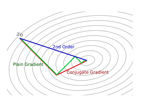
return xk, i, xhistoryThe figure below from [3] depicts how second-order methods like Newton’s method can give better direction and step length than first-order methods like steepest descent. It also foreshadows another method we will cover: conjugate gradient.
Quasi-Newton Methods
The quasi-Newton search directions are an alternative to Newton’s direction: they do not require computation of the Hessian but still attain a superlinear rate of convergence. These directions replace the true Hessian $\nabla^2 f_k$ with an approximation $B_k$ in each step, which infers information about the second derivative of $f$ using changes in the gradient of $f$. They are derived the following way:
\[\begin{align*} \nabla f(x + p) &= \nabla f(x) + \nabla^2 f(x) p + \int_0^1 \big[\nabla^2 f(x + tp) - \nabla^2 f(x)\big] p \D{t} \\ &\quad \: \text{by adding and subtracting } \nabla^2 f(x) p \text{ from Taylor's Theorem} \end{align*}\]As $\nabla f(\cdot)$ is continuous, we also know the following:
\[\int_0^1 \big[\nabla^2 f(x + tp) - \nabla^2 f(x)\big] p \D{t} = O(||p||)\]By setting $x = x_k$ and $p = x_{k+1} - x_k$, we obtain:
\[\nabla f_{k+1} = \nabla f_k + \nabla^2 f_k(x_{k+1} - x_k) + O(||x_{k+1} - x_k||)\]The final integral term definition is eventually dominated by $\nabla^2 f_k(x_{k+1} - x_k)$ as $x_k$ and $x_{k+1}$ lie in a region near the solution $x^*$. This yields the following approximation of the Hessian:
\[\nabla^2 f_k(x_{k+1} - x_k) \approx B_{k+1} = \nabla f_{k+1} - \nabla f_k\]We also want that the approximation $B_{k+1}$, just like the true Hessian, satisfies the secant equation:
\[B_{k+1} s_k = y_k \quad \text{where } s_k = x_{k+1} - x_{k} \text{ and } y_k = \nabla f_{k+1} - \nabla f_k\]The quasi-Newton search direction is then given by using $B_k$ in place of the exact Hessian:
\[p_k = - B_k^{-1} \nabla f_k\]This is the definition of a generic quasi-Newton method; specialized methods, as we shall, see next impose other conditions on the approximation $B_{k+1}$.
Symmetric-Rank-One (SR1) Method
The symmetric-rank-one (SR1) method states that
\[B_{k+1} = B_k + \frac{(y_k - B_k s_k)(y_k - B_k s_k)^T}{(y_k - B_k s_k)^T s_k}\]NOTE: We will not implement this method as BFGS is the more popular and common choice amongst the two for quasi-Newton methods.
BFGS Method
The BFGS method, named after its inventors Broyden, Fletcher, Goldfarb, and Shanno, states that
\[B_{k+1} = B_k - \frac{B_k s_k s_k^T B_k}{s_k^T B_k s_k} + \frac{y_k y_k^T}{y_k^T s_k}\]def bfgs(f, gradient, x0, c1=1e-4, c2=0.9,
algorithm_iters=100, step_length_iters=20, tolerance=1e-5):
"""
Implements BFGS Method as described above.
Per-iteration: 2 Gradient Evaluation, 1 Hessian Approximation, 1 find_step_length()
:returns:
xk: solution reached in `algorithm_iters` or fewer steps
i: num. steps it took to reach `xk`
xhistory: solution trajectory, a list of xi's in each step
"""
# Initialize history, the Hessian, and the first iterate
xhistory = [x0]
I = np.identity(x0.size)
xk = x0
hessian_k = np.identity(x0.size)
# Optimization loop
for i in range(1, algorithm_iters + 1):
# Find gradient and direction for current iterate
gradient_k = gradient(xk)
pk = -hessian_k.dot(gradient_k)
# Get a reasonably good alpha
alpha = find_step_length(f=f,
gradient=gradient,
xk=xk,
alpha=1.0,
pk=pk,
c1=c1,
c2=c2,
iters=step_length_iters)
# Get the next iterate and compute its gradient
xj = xk + alpha * pk
gradient_j = gradient(xj)
# Compute sk and yk as previously defined
sk, yk = xj - xk, gradient_j - gradient_k
# Compute the approximation B_{k+1} for H_{k+1} as previously defined
# NOTE: Here j = k + 1
rho_k = float(1.0 / yk.dot(sk))
hessian_j = (I - rho_k * np.outer(sk, yk)).dot(hessian_k).dot(I - rho_k * np.outer(yk, sk)) + rho_k * np.outer(sk, sk)
# Check for tolerance; if within small distance we finish optimization
if np.linalg.norm(xj - xk) < tolerance:
break
# Update the previous iterate for tolerance-checking and update the history
xk, hessian_k = xj, hessian_j
xhistory.append(xk)
return xk, i, xhistoryConjugate Gradient Method
The conjugate gradient method chooses the direction as
\[p_k = - \nabla f(x_k) + \beta_k p_{k-1}\]where $\beta_k$ is a scalar that ensures that $p_k$ and $p_{k-1}$ are conjugate.
def conjugate_gradient(f, gradient, x0, c1=1e-4, c2=0.1,
                       algorithm_iters=100, step_length_iters=20, tolerance=1e-5):
    """
    Implements Conjugate Gradient Method as described above.
    Per-iteration: 1 Gradient Evaluation, 1 find_step_length()

    :returns:
        xk: solution reached in `algorithm_iters` or fewer steps
        i: num. steps it took to reach `xk`
        xhistory: solution trajectory, a list of xi's in each step
    """
    # Initialize history
    xhistory = [x0]
    xk = x0

    # Initialize the function evaluation, gradient and direction at current iterate
    fk, gradient_k, pk = f(xk), gradient(xk), -gradient(xk)

    # Optimization loop
    for i in range(1, algorithm_iters + 1):
        # Get a reasonably good alpha
        alpha = find_step_length(f=f,
                                 gradient=gradient,
                                 xk=xk,
                                 alpha=1.0,
                                 pk=pk,
                                 c1=c1,
                                 c2=c2,
                                 iters=step_length_iters)

        # Get the next iterate and compute its gradient
        xj = xk + alpha * pk
        gradient_j = gradient(xj)

        # Compute the $\beta$ parameter and get the direction for the next iterate
        beta_j = gradient_j.dot(gradient_j) / gradient_k.dot(gradient_k)
        pj = -gradient_j + beta_j * pk

        # Check for tolerance; if within small distance we finish optimization
        if np.linalg.norm(xj - xk) < tolerance:
            break

        # Update the previous iterate (as well as gradient and direction)
        # for tolerance-checking and update the history
        xk, gradient_k, pk = xj, gradient_j, pj
        xhistory.append(xk)

    return xk, i, xhistory
Experiments
Example Problem: Rosenbrock Function
The Rosenbrock function is a non-convex function introduced by Howard H. Rosenbrock in 1960. It has been widely used in performance testing for optimization algorithms. It is also known as Rosenbrock’s valley or Rosenbrock’s banana function.
The function is defined by:
\[f(x) = f(x_1, x_2) = (a - x_1)^2 + b(x_2 - x_1^2)^2 = a^2 - 2 a x_1 + x_1^2 + b x_2^2 - 2 b x_2 x_1^2 + b x_1^4\]The function has a global minimum at $(x_1, x_2) = (a, a^2)$ where $f(x_1, x_2) = 0$. Usually the parameter setting is: $a = 1$ and $b = 100$.
We can compute the gradient and Hessian of the function:
\[\begin{align*} \nabla f_k &= \begin{bmatrix} 4 b x_1^3 - 4 b x_1 x_2 + 2 x_1 - 2 a \\ 2 b x_2 - 2 b x_1^2 \\ \end{bmatrix} \\ \nabla^2 f_k &= H_k = \begin{bmatrix} 12 b x_1^2 - 4 b x_2 + 2 & -4 b x_1 \\ -4 b x_1 & 2 b\\ \end{bmatrix} \end{align*}\]Now, let’s implement the Rosenbrock function in Python and visualize its surface. The global minimum of the function is inside a long, flat valley. The valley is easily identifiable from the plots as well as mathematically; however, converging to the global minimum is more difficult.
class Rosenbrock(object):
    """
    Implements Rosenbrock function alongside its gradient and Hessian.

    :param (float) a: Parameter `a` in the Rosenbrock definition above; default is 1.0
    :param (float) b: Parameter `b` in the Rosenbrock definition above; default is 100.0
    """
    def __init__(self, a=1.0, b=100.0):
        self.f = lambda x: (a - x[0]) ** 2 + b * (x[1] - x[0] ** 2) ** 2
        self.gradient = lambda x: np.array([
            4 * b * x[0] ** 3 - 4 * b * x[1] * x[0] + 2 * x[0] - 2 * a,
            2 * b * x[1] - 2 * b * x[0] ** 2
        ])
        self.hessian = lambda x: np.array([
            [12 * b * x[0] ** 2 - 4 * b * x[1] + 2, -4 * b * x[0]],
            [-4 * b * x[0], 2 * b]
        ])

    def __call__(self, x, order=0):
        """
        Returns the corresponding (i.e. function, gradient, or Hessian)
        function evaluation based on `order`.

        :param (np.ndarray) x: input array with shape (2, ...) (e.g. np.array([x1, x2]))
        :param (int) order: if 0 returns the Rosenbrock function evaluation at x,
               elif 1 returns the gradient evaluation at x,
               elif 2 returns the Hessian evaluation at x.
        :return: self.f(x) or self.gradient(x) or self.hessian(x)
        """
        assert isinstance(x, np.ndarray) and x.shape[0] == 2
        assert isinstance(order, int)

        if order == 0:
            return self.f(x)
        elif order == 1:
            return self.gradient(x)
        elif order == 2:
            return self.hessian(x)
        else:
            raise NotImplementedError('order=%d is not implemented!' % order)
# Set function parameters and initialize function
a, b = 1.0, 100.0
rosenbrock = Rosenbrock(a=1.0, b=100.0)
# Set plotting parameters and compute x-, y-, and z-axis values
delta = 0.025
xmin, xmax = -1.5, 2.0
ymin, ymax = -0.5, 3.0
x, y = np.arange(xmin, xmax, delta), np.arange(ymin, ymax, delta)
x, y = np.meshgrid(x, y)
z = rosenbrock(np.array([x, y]), order=0)
# First plot for 3D view
fig = plt.figure(figsize=(20, 8))
ax = fig.add_subplot(1, 2, 1, projection='3d')
ax.set_title('3D View of Rosenbrock Function\n', fontsize=18)
ax.set_xlabel(r'$x_1$', fontsize=16)
ax.set_ylabel(r'$x_2$', fontsize=16)
surface = ax.plot_surface(x,
y,
z,
linewidth=0,
cmap=cm.jet,
antialiased=False,
norm=matplotlib.colors.LogNorm())
fig.colorbar(surface, shrink=0.5, aspect=10, label=r'$f(x_1, x_2)$')
ax.view_init(30, 240)
# Second plot for 2D contour view
ax = fig.add_subplot(1, 2, 2)
ax.set_title('2D Contour View of Rosenbrock Function\n', fontsize=18)
ax.set_xlabel(r'$x_1$', fontsize=16)
ax.set_ylabel(r'$x_2$', fontsize=16)
levels = np.array([1e-2, 10**0, 10**1, 10**1.5, 10**2, 10**2.5, 10**3, 10**3.5])
contour = ax.contourf(x,
y,
z,
cmap=cm.jet,
norm=matplotlib.colors.LogNorm(),
levels=levels)
fig.colorbar(contour, shrink=0.5, aspect=10, label=r'$f(x_1, x_2)$')
ax.scatter([a],
[a ** 2],
color='white',
s=200,
label=r'Global Minimum: $(a=1.0, a=1.0)$')
ax.legend(loc='upper left', fontsize=16)
plt.show()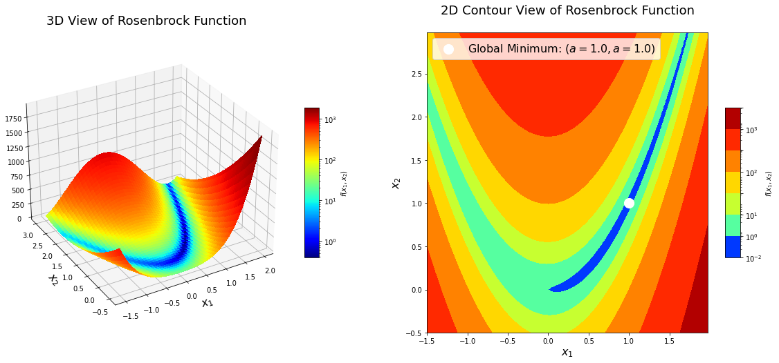
Let’s now try to do optimization (minimization) on the Rosenbrock function we have implemented above using the line search optimization algorithms we have implemented previously.
# Set parameters that will not change (fixed)
tolerance = 1e-6
step_length_iters = 100
solution = (np.array([1.0, 1.0]), np.array([0.0]))

# Set parameters that we will vary
# NOTE: 'Easy' = easy to find the solution for this initial point
# NOTE: 'Medium' = mid-level difficulty problem
# NOTE: 'Hard' = fairly challening problem
# NOTE: Values are inspired from [4]
x0s = {
    'Easy': np.array([0.0, 0.0]),
    'Medium': np.array([2.0, 2.0]),
    'Hard': np.array([-1.2, 1.0])
}
algorithm_iters_all = [2 ** i for i in range(1, 15)]
def experiment(algorithm_iters, x0):
"""
This function carries out the experiment portion of this mini-project. It does:
1. Initializes a logs dictionary with all methods.
2. Using the given `algorithm_iters` and `x0`, calls each method to do
optimization on the Rosenbrock function.
3. Updates logs with
a. Solution `x` found by the current algorithm
b. Number of iterations `niters` it took for the current algorithm
to find the solution `x`
c. Solution path `xhistory` for visualization purposes
"""
logs = {}
method_names = ['Steepest Descent', 'Newton', 'Conjugate Gradient', 'BFGS']
for method_name in method_names:
logs[method_name] = {}
x, niters, xhistory = steepest_descent(rosenbrock.f,
rosenbrock.gradient,
x0,
c1=1e-4,
c2=0.9,
algorithm_iters=algorithm_iters,
step_length_iters=step_length_iters,
tolerance=tolerance)
logs['Steepest Descent']['x'] = x
logs['Steepest Descent']['niters'] = niters
logs['Steepest Descent']['xhistory'] = xhistory
logs['Steepest Descent']['error'] = errors(solution[1], rosenbrock(x, order=0))[0]
x, niters, xhistory = newton(rosenbrock.f,
rosenbrock.gradient,
rosenbrock.hessian,
x0,
c1=1e-4,
c2=0.9,
algorithm_iters=algorithm_iters,
step_length_iters=step_length_iters,
tolerance=tolerance)
logs['Newton']['x'] = x
logs['Newton']['niters'] = niters
logs['Newton']['xhistory'] = xhistory
logs['Newton']['error'] = errors(solution[1], rosenbrock(x, order=0))[0]
x, niters, xhistory = conjugate_gradient(rosenbrock.f,
rosenbrock.gradient,
x0,
c1=1e-4,
c2=0.1,
algorithm_iters=algorithm_iters,
step_length_iters=step_length_iters,
tolerance=tolerance)
logs['Conjugate Gradient']['x'] = x
logs['Conjugate Gradient']['niters'] = niters
logs['Conjugate Gradient']['xhistory'] = xhistory
logs['Conjugate Gradient']['error'] = errors(solution[1], rosenbrock(x, order=0))[0]
x, niters, xhistory = bfgs(rosenbrock.f,
rosenbrock.gradient,
x0,
c1=1e-4,
c2=0.9,
algorithm_iters=algorithm_iters,
step_length_iters=step_length_iters,
tolerance=tolerance)
logs['BFGS']['x'] = x
logs['BFGS']['niters'] = niters
logs['BFGS']['xhistory'] = xhistory
logs['BFGS']['error'] = errors(solution[1], rosenbrock(x, order=0))[0]
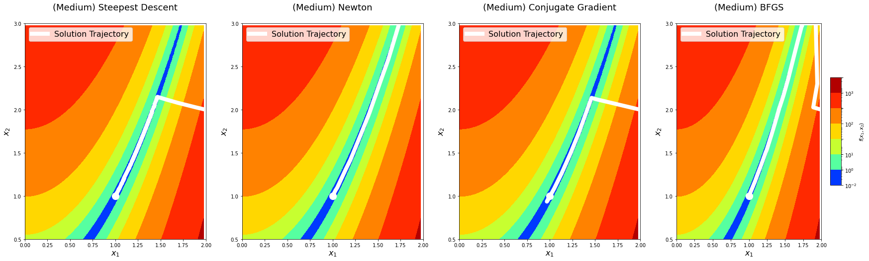
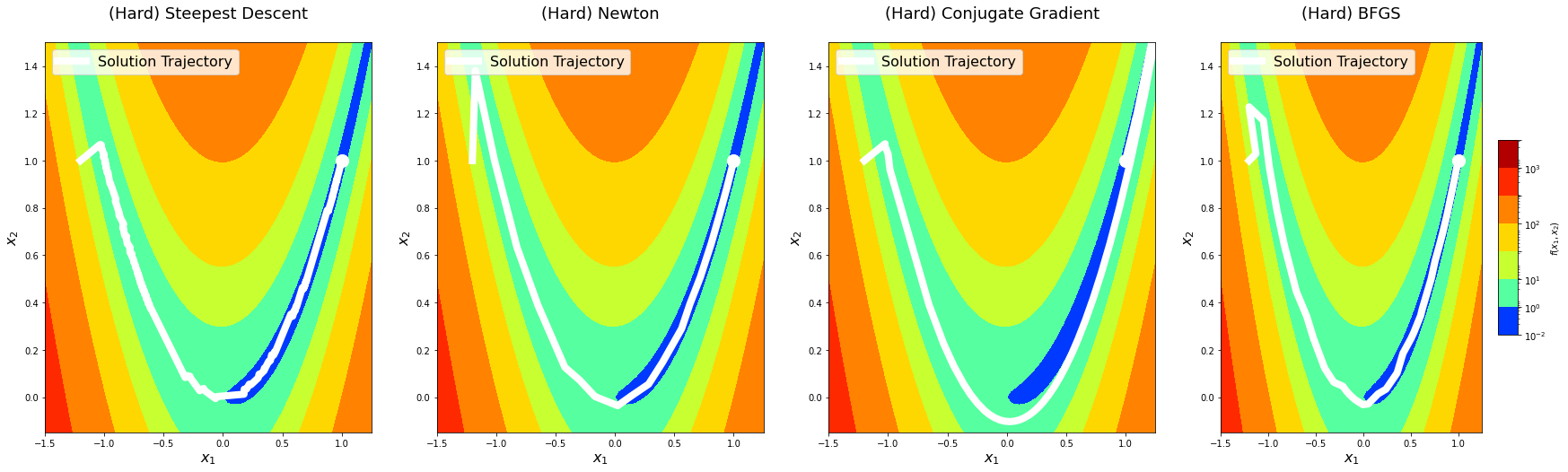
return logsBefore doing deeper analysis on the performance and convergence of the algorithms, let’s first plot the solution paths of each optimization algorithm with algorithm_iters = 1024 on the predefined points. This is mostly for fun, but it might also provide an additional perspective.
for level in x0s:
    logs = experiment(algorithm_iters=1024, x0=x0s[level])

    ### Second plot for 2D contour view ###
    fig = plt.figure(figsize=(30, 8))

    for i, method_name in enumerate(logs):
        ax = fig.add_subplot(1, len(logs), i + 1)
        ax.set_title('(%s) %s\n' % (level, method_name), fontsize=18)
        ax.set_xlabel(r'$x_1$', fontsize=16)
        ax.set_ylabel(r'$x_2$', fontsize=16)
        levels = np.array([1e-2, 10**0, 10**1, 10**1.5, 10**2, 10**2.5, 10**3, 10**3.5])
        contour = ax.contourf(x,
                              y,
                              z,
                              cmap=cm.jet,
                              norm=matplotlib.colors.LogNorm(),
                              levels=levels)
        ax.scatter([a], [a ** 2], color='white', s=200)

        xhistory = np.vstack(logs[method_name]['xhistory'])
        ax.plot(xhistory[:, 0],
                xhistory[:, 1],
                linestyle='-',
                linewidth=8,
                color='white',
                label='Solution Trajectory')
        ax.legend(loc='upper left', fontsize=16)

        if level == 'Hard':
            ax.set_xlim(-1.5, 1.25)
            ax.set_ylim(-0.15, 1.5)
        elif level == 'Medium':
            ax.set_xlim(0.0, 2.0)
            ax.set_ylim(0.5, 3.0)
        elif level == 'Easy':
            ax.set_xlim(0.0, 1.1)
            ax.set_ylim(-0.1, 1.5)

    fig.colorbar(contour, shrink=0.5, aspect=10, label=r'$f(x_1, x_2)$')
    plt.show()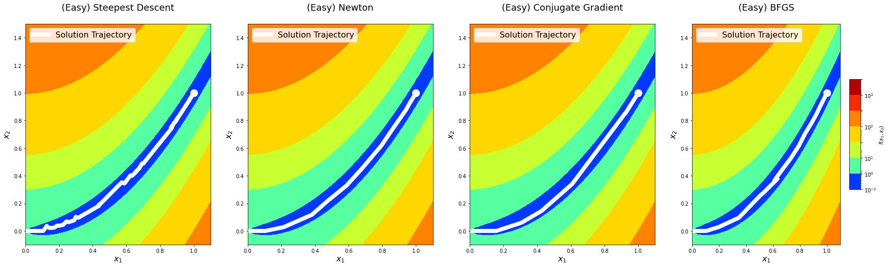
Let’s now vary algorithm_iters and plot error as a function of the number of iterations. We will do this across different starting points with different difficulty levels. This will give us an idea of the convergence rate and relative performance of the optimization algorithms we have implemented.
fig, ax = plt.subplots(1, len(x0s), figsize=(20, 8))

for i, level in enumerate(x0s):
    ax[i].set_title('(%s) Error vs. Num. Iterations' % level)
    ax[i].set_xlabel('Num. Iterations')
    ax[i].set_ylabel('Absolute Error')
    ax[i].grid()

    x = algorithm_iters_all
    y_steepest, y_newton, y_conjugate, y_bfgs = [], [], [], []


    for algorithm_iters in algorithm_iters_all:
        logs = experiment(algorithm_iters=algorithm_iters, x0=x0s[level])

        y_steepest.append(logs['Steepest Descent']['error'])
        y_newton.append(logs['Newton']['error'])
        y_conjugate.append(logs['Conjugate Gradient']['error'])
        y_bfgs.append(logs['BFGS']['error'])


    ax[i].loglog(x, y_steepest, color='blue', label='Steepest Descent')
    ax[i].plot(x, y_newton, color='red', label='Newton')
    ax[i].plot(x, y_conjugate, color='purple', label='Conjugate Gradient')
    ax[i].plot(x, y_bfgs, color='gold', label='BFGS')

    if i == len(x0s) // 2:
        ax[i].legend(loc='upper right', fontsize=12)

plt.show()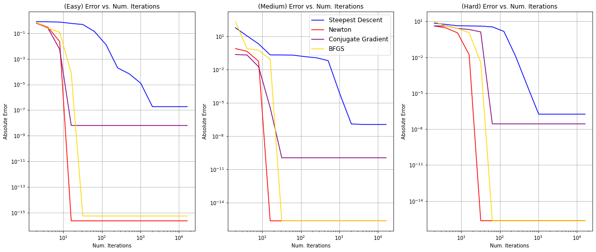
Analysis
Solution Trajectory Visualization
The solution trajectory visualizations show that the steepest descent method is the noisiest, whereas others are reasonably smoother. This aligns well with the idea that Newton’s method and other methods that use information from the second-derivative get better gradient directions and step sizes. We notice that the conjugate gradient method overshoots the minima on the hard level the first time it comes around. We see something similar with the BFGS method on the medium level.
Convergence Rate and Performance
First of all, we notice that Newton’s method, conjugate gradient, and BFGS all converge between $10^1$ and $10^2$ in all levels, whereas steepest descent converges much later, between $10^3$ and $10^4$. Moreover, steepest descent always converges at a higher absolute error when compared to other algorithms. This supports our previous claims that steepest ascent has the advantage of only requiring calculation of the gradient but not of second derivatives, yet it can be painfully slow on difficult problems. On the other hand, Newton’s method and quasi-Newton methods reach superlinear convergence but are more computationally expensive. They also acquire better performance compared to steepest descent as previously discussed.
Moreover, Newton’s method has the highest convergence rate and achieves the best absolute error overall. The second-best convergence rate and absolute error overall is the quasi-Newtonian BFGS method. BFGS and other quasi-Newton methods do not require computation of the Hessian but still attain a superlinear rate of convergence. Our graph supports this as the rate of convergence is comparable. The rate of convergence of the conjugate gradient method follows closely after; however, the performance of this method in terms of the absolute error is poor compared to Newton’s method and BFGS. This makes sense: the conjugate descent method tries to accelerate the convergence rate of steepest descent while avoiding the high computational cost of Newton’s method and therefore falls right in between.
References
[1] Jorge Nocedal, Stephen J. Wright, Numerical Optimization (2nd Edition), Springer
[2] University of Stuggart, Introduction to Optimization, Marc Toussaint, Lecture 02
[3] University of Stuggart, Introduction to Optimization, Marc Toussaint, Lecture 04
[4] algopy documentation
[5] Carnegie Mellon University, Convex Optimization, Aarti Singh and Pradeep Ravikumar
[6] Columbia University, APMA E4300: Computational Math: Introduction to Numerical Methods, Marc Spiegelman
NOTE: The majority of the material covered here is inspired and adapted from [1].